Dataset
HapMap
The goal of the International HapMap Project was to determine the common patterns of DNA sequence variation in the human genome and to make this information freely available in the public domain. An international consortium developed a map of these patterns across the genome by determining the genotypes of one million or more sequence variants, their frequencies and the degree of association between them, in DNA samples from populations with ancestry from parts of Africa, Asia and Europe. The HapMap has become an important tool for researchers to use to find genes that affect health, disease, and response to drugs and environmental factors.
The DNA sequence of any two people is 99.9 percent identical. The variations, however, may greatly affect an individual's disease risk. Sites in the DNA sequence where individuals differ at a single DNA base are called Single Nucleotide Polymorphisms (SNPs). Sets of nearby SNPs on the same chromosome are inherited in blocks. This pattern of SNPs on a block is a haplotype. Blocks may contain a large number of SNPs, but a few SNPs (i.e. tag SNPs) are enough to uniquely identify the haplotypes in a block. The HapMap is a map of these haplotype blocks and the specific SNPs that identify the haplotypes are called tag SNPs.
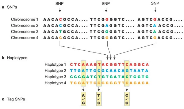
a) SNPs. Shown is a short stretch of DNA from four versions of the same chromosome region in different people. Most of the DNA sequence is identical in these chromosomes, but three bases are shown where variation occurs. Each SNP has two possible alleles; the first SNP in panel a has the alleles C and T.
b) Haplotypes. A haplotype is made up of a particular combination of alleles at nearby SNPs. Shown here are the observed genotypes for 20 SNPs that extend across 6,000 bases of DNA. Only the variable bases are shown, including the three SNPs that are shown in panel a. For this region, most of the chromosomes in a population survey turn out to have haplotypes 1–4.
c) Tag SNPs. Genotyping just the three tag SNPs out of the 20 SNPs is sufficient to identify these four haplotypes uniquely. For instance, if a particular chromosome has the pattern A–T–C at these three tag SNPs, this pattern matches the pattern determined for haplotype 1. Note that many chromosomes carry the common haplotypes in the population.
HapMap3 genotype data in plink format
This tutorial is based on the freely available data in plink format from the third phase of the International HapMap project (HapMap 3). The plink genotype files can be obtained from https://ftp.ncbi.nlm.nih.gov/hapmap/genotypes/hapmap3_r3/plink_format/. Alleles in this dataset are expressed in the forward (+) strand of the reference human genome (NCBI build 36 or UCSC hg18).
Simulated binary outcome measure
To be able to illustrate all analysis steps using realistic genetic data, Marees et al. 2018 simulated a dataset (N = 207) with a binary outcome measure using the publicly available data from the International HapMap Project. For simplicity reasons in this tutorial we focus on a binary outcome measure, and thus this tutorial is not ideal if you are working with quantitative outcome measures. Most GWAS studies are performed on genetically homogenous population, in which population outliers are removed. The HapMap data, used in this tutorial, contains multiple distinct populations, which makes it problematic for analysis. In order to ensure that population used in this tutorial is relatively homogenous only the EUR individuals from the HapMap project (i.e. only Utah residents with ancestry from Northern and Western Europe (CEU)) were included in the data refered to as hapmap. Because of the relatively small sample size of the HapMap data, genetic effect sizes in these simulations were set at values larger than usually observed in genetic studies of complex traits. It is important to note that larger sample sizes (e.g., at least in the order of thousands but likely even tens or hundreds of thousands) will be required to detect genetic risk factors of complex traits. The HapMap data with a simulated phenotypic trait can be downloaded from https://github.com/MareesAT/GWA_tutorial/.
1000 Genomes Project
In this tutorial we are going to check for population stratification in our HapMap subset dataset by anchoring it with the help of the 1000 Genomes Project (1KGP). This will help us to determine if there is population stratification in our dataset or if there are any outliers.
The 1KGP created a catalogue of common human genetic variation, using openly consented samples from people who declared themselves to be healthy. The goal of the 1000 Genomes Project was to find common genetic variants with frequencies of at least 1% in the populations studied. The 1000 Genomes Project took advantage of developments in sequencing technology, which sharply reduced the cost of sequencing. The 1000 Genomes Project ran between 2008 and 2015, creating the largest public catalogue of human variation and genotype data. The reference data resources generated by the project remain heavily used by the biomedical science community.
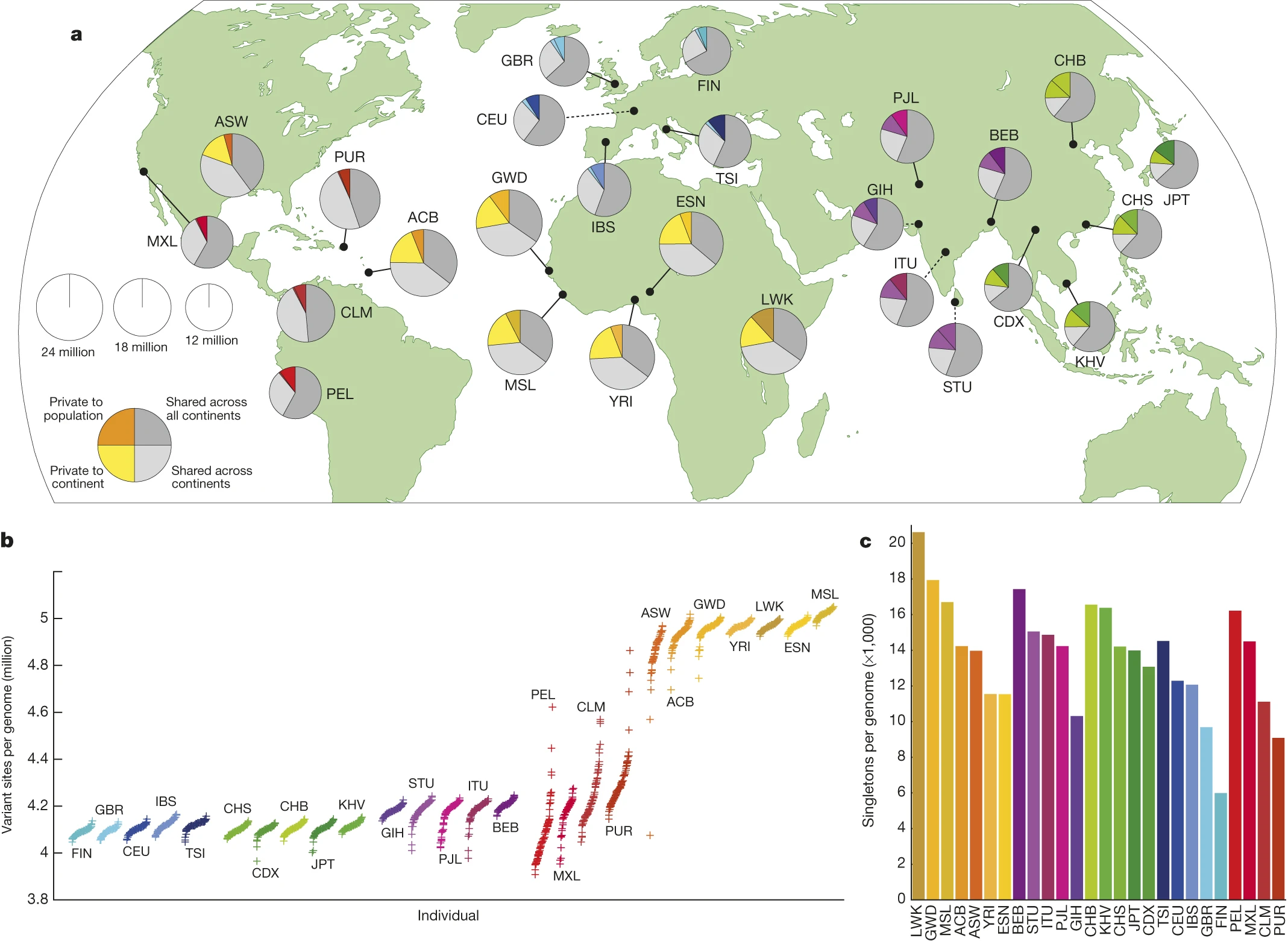
a) Polymorphic variants within sampled populations. The area of each pie is proportional to the number of polymorphisms within a population. Pies are divided into four slices, representing variants private to a population (darker colour unique to population), private to a continental area (lighter colour shared across continental group), shared across continental areas (light grey), and shared across all continents (dark grey). Dashed lines indicate populations sampled outside of their ancestral continental region. b) The number of variant sites per genome. c) The average number of singletons per genome.
Publications:
Pilot
A map of human genome variation from population-scale sequencing Nature 467, 1061–1073 (28 October 2010)
Phase 1
An integrated map of genetic variation from 1,092 human genomes Nature 491, 56–65 (01 November 2012)
Phase 3
A global reference for human genetic variation Nature 526, 68–74 (01 October 2015)
An integrated map of structural variation in 2,504 human genomes Nature 526, 75–81 (01 October 2015)
1KGP data
The 1KGP vcf files containing 629 individuals from different populations could be downloaded using the ftp link from an official International Genome Sample Resource (IGSR) webpage. Detailed preparation steps for 1kgp data for this tutorial can be found in the section "1KGP preparation".
Copying data for tutorials
Copy tutorials and exercises in your home directory and move to gwas_exercises/out from where you will execute all of the commands from this tutorial.
cp -r /opt/evop/public/BIOINFORMATICS/gwas_exercises ~

cd ~/gwas_exercises/out
The gwas_intro directory contains a few subdirectories that will help us to keep our tutorial and output organized.
data: contains data necessary for this tutorial.scripts: contains R scripts that we will use to visualize the output.plots: will store plots produces by R scripts.out: will store final and all intermediate files of this tutorial.