Association analyses
After QC and calculation of MDS components, the data are ready for subsequent association tests. Depending on the expected genetic model of the trait or disease of interest and the nature of the phenotypic trait studied, the appropriate statistical test can be selected.
Plink offers one degree of freedom (1 df) allelic tests in which the trait value, or the log-odds of a binary trait, increases or decreases linearly as a function of the number of risk alleles (minor allele a vs. major allele A).
In addition, non-additive tests are available, for instance:
- the genotypic association test (2 df: aa vs. Aa vs. AA),
- the dominant gene action test (1 df: aa & Aa vs. AA), and
- the recessive gene action test (1 df: aa vs. Aa & AA).
However, non-additive tests are not widely applied, because the statistical power to detect non-additivity is low in practice. More complex analyses (e.g., Cox regression analysis and cure models) can be performed by using R-based “plug-in” functions in plink.
Association analyses for quantitative traits

Within plink, the association between SNPs and quantitative outcome measures (e.g. the height; the number of alcoholic beverages consumed per week...) can be tested with the options --assoc and --linear.
- The
--assocoption will automatically detect a quantitative outcome measure (i.e., values other than 1, 2, 0, or missing) and it will perform an asymptotic version of the usual Student's t test to compare two means. This option does not allow the use of covariates. - The
--linearoption performs a linear regression analysis with each individual SNP as a predictor. This option allows the the inclusion covariates but it is somewhat slower than the--assocoption.
Association analyses for binary traits

Within plink, the association between SNPs and a binary outcome (e.g. disliking vs. liking cilantro; alcohol dependent patients vs. healthy controls...) can be tested with the options --assoc or --logistic.
- The
--assocoption performs a X^2 test of association that does not allow the inclusion of covariates. - The
--logisticoption performs a logistic regression analysis that allows the inclusion of covariates.
The --logistic option is more flexible than the --assoc option, yet it comes at the price of increased computational time.
In this tutorial, we will focus only on binary traits (e.g. disliking vs. liking cilantro).
Note
The default phenotype codes in plink are:
1 = unaffected
2 = affected
0 or −9 = missing
--assoc
Given a case/control phenotype, --assoc writes the results of a 1df chi-square allelic test to .assoc file. This output file contains a header line, and then one line per variant with the following fields:
| CHR | Chromosome code |
| SNP | Variant identifier |
| BP | Base-pair coordinate |
| A1 | Allele 1 (usually minor) |
| F_A | Allele 1 frequency among cases |
| F_U | Allele 1 frequency among controls |
| A2 | Allele 2 |
| CHISQ | Allelic test chi-square statistic. |
| P | Allelic test p-value |
| OR | odds(allele 1 in case) / odds(allele 1 in control) |
cd ~/gwas_exercises/out

plink --bfile hapmap_gwa --assoc --out assoc_results
Note
The --assoc option does not allow to correct covariates such as principal components (PCs) or MDS components, which makes it less suited for association analyses.
--logistic
given a case/control phenotype and some covariates --logistic performs logistic regression. We will be using 10 MDS components calculated from the previous tutorial as covariates in this logistic analysis. This output file contains a header line, and then one line per variant with the following fields:
| CHR | Chromosome code. Not present with 'no-snp' modifier. |
| SNP | Variant identifier. Not present with 'no-snp'. |
| BP | Base-pair coordinate. Not present with 'no-snp'. |
| A1 | Allele 1 (usually minor). Not present with 'no-snp'. |
| TEST | Test identifier |
| NMISS | Number of observations (nonmissing genotype, phenotype, and covariates) |
| OR | Odds Ratio (--logistic without 'beta') |
| STAT | T-statistic |
| P | Asymptotic p-value for t-statistic |
plink --bfile hapmap_gwa --covar hapmap_gwa.covar --logistic --hide-covar --out logistic_results
Note
--hide-covar removes covariate-specific lines from the main report.
Remove NA values, those might give problems generating plots in next steps
awk '!/'NA'/' logistic_results.assoc.logistic > logistic_results.assoc_2.logistic
The results obtained from these GWAS analyses will be visualized in the last step. This will also show if the data set contains any genome-wide significant SNPs.
Multiple testing
Modern genotyping arrays can genotype millions of markers, which generates a large number of tests, and thus, a considerable multiple testing burden. SNP imputation may further increase the number of tested associations. Various simulations have indicated that the widely used genome-wide significance threshold of 5×10⁻⁸ for studies on European populations adequately controls for the number of independent SNPs in the entire genome, regardless of the actual SNP density of the study. When testing African populations, more stringent thresholds are required due to the greater genetic diversity among those individuals.
Three widely applied alternatives for determining genome-wide significance are the use of Bonferroni correction, Benjamini–Hochberg false discovery rate (FDR), and permutation testing.
-
The Bonferroni correction aims to control the probability of having at least one false positive finding. It calculates the adjusted p value threshold with the formula
0.05/n, withnbeing the number of SNPs tested. However, as stated previously, many SNPs are correlated, due to Linkage Disequilibrium (LD) and are thus by definition not independent. Therefore, this method is often too conservative and leads to an increase in the proportion of false negative findings. -
FDR controls the expected proportion of false positives among all signals with an FDR value below a fixed threshold, assuming that SNPs are independent. This method is less conservative than Bonferroni correction. It should be noted that controlling for FDR does not imply any notion of statistical significance; it is merely a method to minimize the expected proportion of false positives, for example, for follow-up analyses. Moreover, this method has its own limitation as SNPs and thus p values are not independent whereas this is an assumption of the FDR method.
-
Permutation methods can be used to deal with the multiple testing burden. To calculate permutation-based p values, the outcome measure labels are randomly permuted multiple (e.g., 1,000–1,000,000) times which effectively removes any true association between the outcome measure and the genotype. For all permuted data sets, statistical tests are then performed. This provides the empirical distribution of the test-statistic and the p values under the null hypothesis of no association. The original test statistic or p value obtained from the observed data is subsequently compared to the empirical distribution of p values to determine an empirically adjusted p value.
--adjust
To easily apply Bonferroni and FDR correction, plink offers the option --adjust that generates output in which the unadjusted p value is displayed, along with p values corrected with various multiple testing correction methods.
plink --bfile hapmap_gwa --assoc --adjust --out adjusted_assoc_results
This file gives a Bonferroni corrected p-value, along with FDR and others.
--mperm
To perform permutation test in plink, options --assoc and --mperm can be combined to generate two p values:
- EMP1, the empirical p value (uncorrected), and
- EMP2, the empirical p value corrected for multiple `testing.
This procedure is computationally intensive, especially if many permutations are required, which is necessary to calculate very small p values accurately.
To reduce computational time we will perform this test only on a subset of the SNPs from chromosome 22.
Generate subset of SNPs from chromosome 22
plink --bfile hapmap_gwa --chr 22 --make-bed --out hapmap_gwa_chr22subset
Perform 1000000 perrmutations
plink --bfile hapmap_gwa_chr22subset --assoc --mperm 1000000 --out hapmap_gwa_chr22subset
Order your data, from lowest to highest p-value and check ordered permutation results
sort -gk 4 hapmap_gwa_chr22subset.assoc.mperm | head
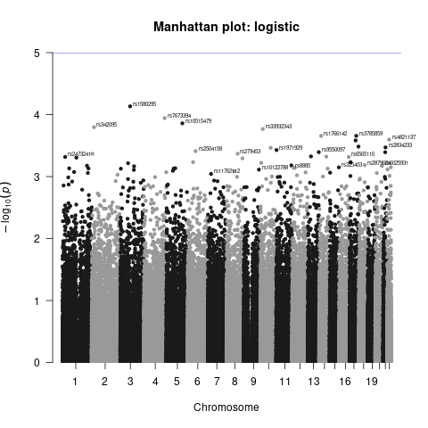
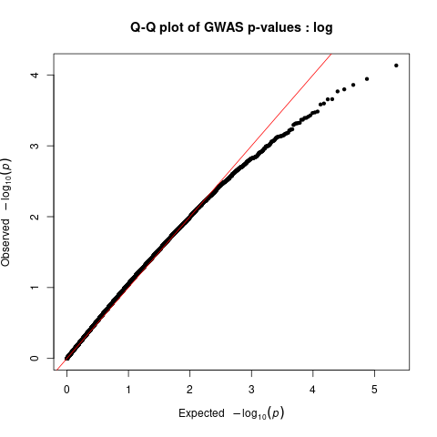
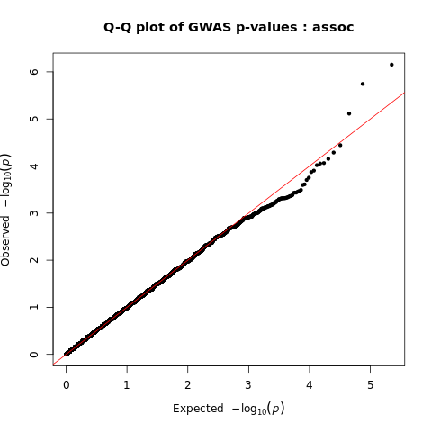
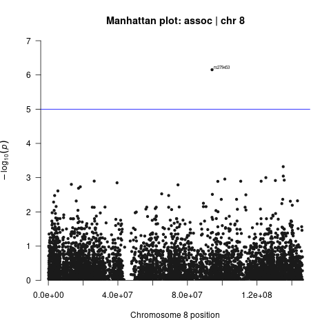
Generate Manhattan and QQ plots
We will visualize the output of the association analysis with Manhattan plot and quantile–quantile plot using R script manhattan_qq.R.
Rscript --vanilla ../scripts/manhattan_qq.R
Manhattan plots show us the significance of each variant’s association with a phenotype (e.g. disliking vs. liking cilantro). Each dot represents a single-nucleotide polymorphism (SNP). SNPs are ordered on the x axis according to their genomic position. y axis represents strength of their association measured as –log10 transformed P values. Blue line marks genome-wide significance threshold of P < 5 × 10⁻⁸.
Quantile–quantile plots show us distribution of expected P values under a null model of no significance versus observed P values. Expected –log10 transformed P values (x axis) for each association are plotted against observed values (y axis) to visualize the enrichment of association signal. Deviation from the expectation under the null hypothesis (red line) indicates the presence of either true causal effects or insufficiently corrected population stratification. In the case of true causal effects, one would expect to observe this deviation mostly at the right side of the plot, whereas population stratification causes the deviation to start closer to the origin. In this case, BMI is extremely polygenic and the genome-wide association study (GWAS) was highly powered, which may also cause the deviation to start close to the origin, making it difficult to visually spot stratification. LDSC may be used to assess whether this inflation is due to bias or polygenicity.