Quality Control

You can find a thorough theoretical explanation of all QC steps in A tutorial on conducting Genome-Wide-Association Studies: Quality control and statistical analysis.

A vital step that should be part of any GWAS is the use of appropriate QC. Without extensive QC, GWAS will not generate reliable results because raw genotype data are inherently imperfect. Errors in the data can arise for numerous reasons, for example, due to poor quality of DNA samples, poor DNA hybridization to the array, poorly performing genotype probes, and sample mix-ups or contamination.

The QC steps consist of filtering out of SNPs and individuals based on the following:

• missingness
• inconsistencies in assigned and genetic sex of subjects (sex discrepancy)
• minor allele frequency (MAF)
• deviations from Hardy–Weinberg equilibrium (HWE)
• heterozygosity rate
• relatedness
• population stratification

Before starting tutorial let's change the current working directory to gwas_exercises/out from which we will run majority of commans.

cd ~/gwas_exercises/out

Missingness

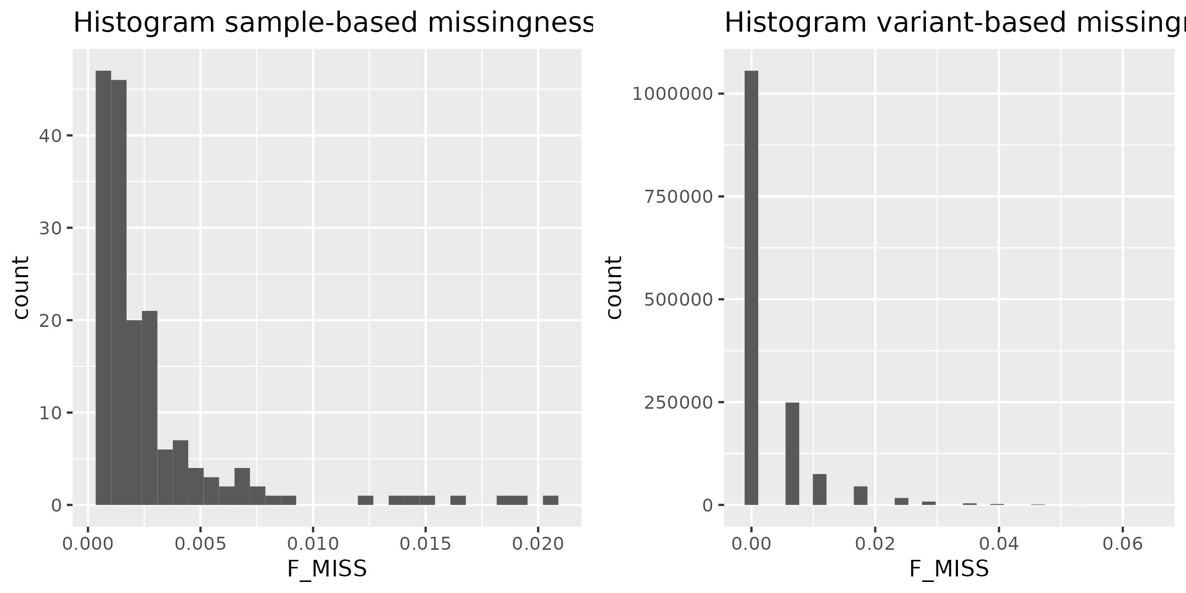
First we can investigate missingness per individual and per SNP by making histograms. To do so we will use --missing in plink.

plink --bfile ../data/hapmap --missing --out hapmap

This will output two files:
- .imiss contains information about the proportion of missing SNPs per individual ("i" - individual)
- .lmiss contains information about the proportion of missing individuals per locus ("l" - locus).

Now we can generate in R histograms to visualize the missingness results. We will use R script called hist_miss.R. This script will produce histograms for both imiss and lmiss files and output it as hist_miss.png in ~/gwas_exercises/plots. Once you run the R script take a look at the figure.

Rscript --vanilla ../scripts/hist_miss.R

In the next step we can delete SNPs (--geno) and individuals (--mind) with missingness >0.2 (which is already satisfied in our dataset, but for demonstration purposes we will run the command).

plink --bfile ../data/hapmap --geno 0.2 --mind 0.2 --make-bed --out hapmap_1

Sex check

In the next step we can check for sex discrepancies between genetic sex and reported sex. To do so we can use --check-sex to identify individual with discordant sex information. The --check-sex will calculate the F value based on the X chromosome inbreeding (homozygosity) estimate.
- Females should have F value < 0.2
- Males should have F value > 0.8

Individuals who do not fulfil these requirements are flagged with "PROBLEM" by plink.

plink --bfile hapmap_1 --check-sex --out hapmap_1

Generate plots to visualize the sex-check results.

Rscript --vanilla ../scripts/sex_check.R

Inspection of sex_check.png plots shows that there is one individual indicated as female based on the pedsex with the F value of 0.99, and thus showing sex discrepancy.

Depending on our main goal we can either choose to remove individuals with sex discrepeancy, or we can impute the sex of individuals based on the genotype information (--impute-sex). In our case, we will stick to more conservative approach and exclude individuals that showed sex discrepancy.

To delete individuals with sex discrepancy we will first make a list of problematic individuals based on .sexcheck file.

awk '{if ($5 == "PROBLEM") print $1, $2}' hapmap_1.sexcheck > hapmap_1.sexcheck_problem

In the next step, we can use plink to --remove those individuals from our dataset.

plink --bfile hapmap_1 --remove hapmap_1.sexcheck_problem --make-bed --out hapmap_2

plink --bfile hapmap_1 --impute-sex --make-bed --out hapmap_2

Autosomes

In this tutorial we will focus on autosomal SNPs. To keep only SNPs located on autosomal chromosomes (i.e. chromosomes 1-22) we can use --autosomes in plink.

plink --bfile hapmap_2 --autosome --make-bed --out hapmap_3

MAF

Minor allele frequency (MAF) is the frequency of the least often occurring allele at a specific location. SNPs with a low MAF are rare, and most studies are underpowered to detect associations between SNP with low MAF and phenotype. These SNPs are also more prone to genotyping errors, and therefore they are often excluded. The appropriate MAF threshold depends on the sample size. Larger sample sizes can use lower MAF thresholds when compared with smaller sample sizes. Commonly used MAF threshold for large sample sizes (N = 100.000) is 0.001, and for moderate sample sizes (N = 10.000) is 0.05.

We can use plink's --freq to get a minor allele frequency report .frq.

plink --bfile hapmap_3 --freq --out hapmap_3

We can then use this .frq report to generate a plot of the MAF distribution using the R script maf_check.R.

Rscript --vanilla ../scripts/maf_check.R

In the next step we can remove SNPs with a low MAF frequency using --maf and desired threshold (in our case 0.05).

plink --bfile hapmap_3 --maf 0.05 --make-bed --out hapmap_4

HWE

The Hardy–Weinberg principle states that allele and genotype frequencies in a population will remain constant from generation to generation in the absence of other evolutionary influences (i.e. genetic drift, mate choice, assortative mating, natural selection, sexual selection, mutation, gene flow, meiotic drive, genetic hitchhiking, population bottleneck, founder effect, inbreeding and outbreeding depression).

Violation of the HWE indicates that genotype frequencies are significantly different from expectations (e.g., if the frequency of allele Y = 0.7 and the frequency of allele y = 0.3; the expected frequency of genotype Yy is 2 x 0.7 x 0.3 = 0.42) and the observed frequency should not be significantly different. In GWAS, it is generally assumed that extreme deviations from HWE are the result of genotyping errors. The HWE thresholds in cases are often less stringent than those in controls, as the violation of the HWE law in cases can be indicative of true genetic association with disease risk.

For binary traits it is suggested to exclude variants with HWE p value < 1e−10 in cases, and HWE p value < 1e−6 in controls. For quantitative traits, we recommend excluding variants with HWE p value <1e‐6.

In the next step we will excludes SNPs which deviate from Hardy–Weinberg equilibrium (HWE). We will assume that poor genotype calling is the main reason for huge genotype frequencies deviations from HWE.

First we will create HWE report .hwe for each SNP in our dataset using plink's --hardy.

plink --bfile hapmap_4 --hardy --out hapmap_4

Next we will use R to check the distribution of HWE p-values for all SNPs.
R script hwe.R will produce hwe_plots.png containing 3 different plots.
1) Scatter plots of Observed "O(HET)" vs Expected "E(HET)" heterozygosities separately for affected (AFF), and unaffected (UNAFF), and all (ALL) individuals.
2) Histogram of HWE p-values.
3) Zoom-in-histogram for strongly deviating SNPs with HWE p-value below 0.00001.

Rscript --vanilla ../scripts/hwe.R

Finally, we can use --hwe to exclude SNPs deviating from HWE. By default the --hwe option in plink only filters for controls. It is recommended to remove SNPs that have a deviation from HWE p < 10-6 in controls.

plink --bfile hapmap_4 --hwe 10e-6 --make-bed --out hapmap_5

LD pruning

As GWAS typically involve testing hundreds of thousands or even millions of genetic variants for association with a trait of interest, performing LD pruning can help to reduce the number of genetic variants included in the analysis while retaining most of the information captured by the remaining variants. This can reduce the number of multiple testing corrections required and improve the statistical power to detect true associations.

Additionally, LD pruning can help to remove genetic variants that are in high LD with each other, which are likely to provide redundant information in the analysis. This can reduce the risk of false positives and improve the interpretability of the results.

However, it is important to note that LD pruning may not always be necessary or appropriate for all GWAS datasets. The optimal parameters for LD pruning may vary depending on the genetic structure and sample size of the dataset, as well as the research question and hypothesis being tested. It is therefore important to carefully consider the potential benefits and drawbacks of LD pruning in the context of your specific GWAS analysis.

To generate a list of SNPs that are not highly correlated with each other, we will prune the SNPs using --indep-pairwise 50 5 0.2. In this example, we use the --indep-pairwise flag to perform LD pruning, where the parameters 50, 5, and 0.2 refer to the window size, the step size, and the threshold for the multiple correlation coefficient r² LD values, respectively. These values can be adjusted based on your dataset and research question.

plink --bfile hapmap_5 --indep-pairwise 50 5 0.2 --out hapmap_5

Next we can use --indep-pairwise output files (.prune.in and .prune.out) as input for --extract/--exclude to create file containing pruned set of SNPs.

plink --bfile hapmap_5 --extract hapmap_5.prune.in --make-bed --out hapmap_6

Heterozygosity

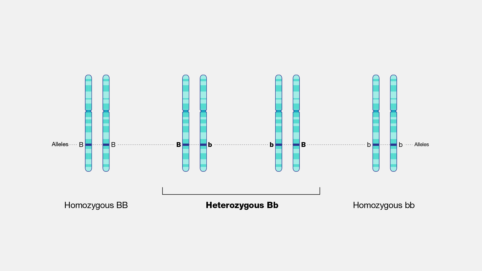
Heterozygosity is the carrying of two different alleles of a specific SNP. The heterozygosity rate of an individual is the proportion of heterozygous genotypes, and thus it is recommended to remove individuals who deviate ±3 SD from the samples' heterozygosity rate mean. - High levels of heterozygosity within an individual might be an indication of low sample quality. - Low levels of heterozygosity within an individual might be due to inbreeding.

It is recommended to perform checks for heterozygosity on a set of SNPs which are not highly correlated (i.e. LD pruned). We can use flag --het to compute observed and expected autosomal homozygous genotype counts for each sample, and method-of-moments F coefficient estimates.

plink --bfile hapmap_6 --het --out hapmap_6

Once we calculated heterozygosity, we can use R script het_check.R to generate a list of individuals who deviate more than 3 standard deviations from the mean F in file hapmap_6.het_fail_ind. This script will also plot histogram for F in file hist_F.png.

Rscript --vanilla ../scripts/het_check.R

Finally after inspecting the plot we can remove individuals that are heterozygosity rate outliers.

plink --bfile hapmap_6 --remove hapmap_6.het_fail_ind --make-bed --out hapmap_7

Relatedness

It is essential to check datasets you analyse for cryptic relatedness as they can interfere with the association analysis.

If you have a family‐based sample (e.g., parent‐offspring), you do not need to remove related pairs but the statistical analysis should take family relatedness into account.

However, for a population based sample (withouth known relatives) you can use plink's --genome to explore genetic relatedness among individuals based on Pi-hat and IBD values.

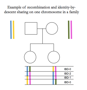
IBD (identity-by-descent) is a measure of the probability that two individuals share a common ancestor for a given segment of DNA. In plink, IBD is estimated using a method called identity-by-state (IBS), which compares the genotypes of two individuals at each SNP marker to determine if they match. If the genotypes match, it suggests that the two individuals share a common ancestor for that segment of DNA, but not necessarily recent ancestry.

Pi-hat is defined as the proportion of alleles that are identical by descent (IBD) between two individuals, and it is calculated as: P(IBD=2) + 0.5 * P(IBD=1). Pi-hat values range from 0 to 1, with values closer to 1 indicating higher levels of genetic similarity.

Let's calculate IBD and Pi-hat:

plink --bfile hapmap_7 --genome --out hapmap_7

This command will output hapmap_7.genome which contains pairwise information about relatedness between pairs of individuals. Important columns for understanding the output are:
- Z0 = P(IBD=0) - probability that at a given locus 0 alleles are identical by descent.
- Z1 = P(IBD=1) - probability that at a given locus 1 allele is shared.
- Z2 = P(IBD=2) - probability that at a given locus 2 alleles are shared.
- PI_HAT = P(IBD=2) + 0.5*P(IBD=1) - Proportion of alleles that are IBD.

In the next step we can use R script genome.R to generate plots to assess the relationship between individuals.

Rscript --vanilla ../scripts/genome.R

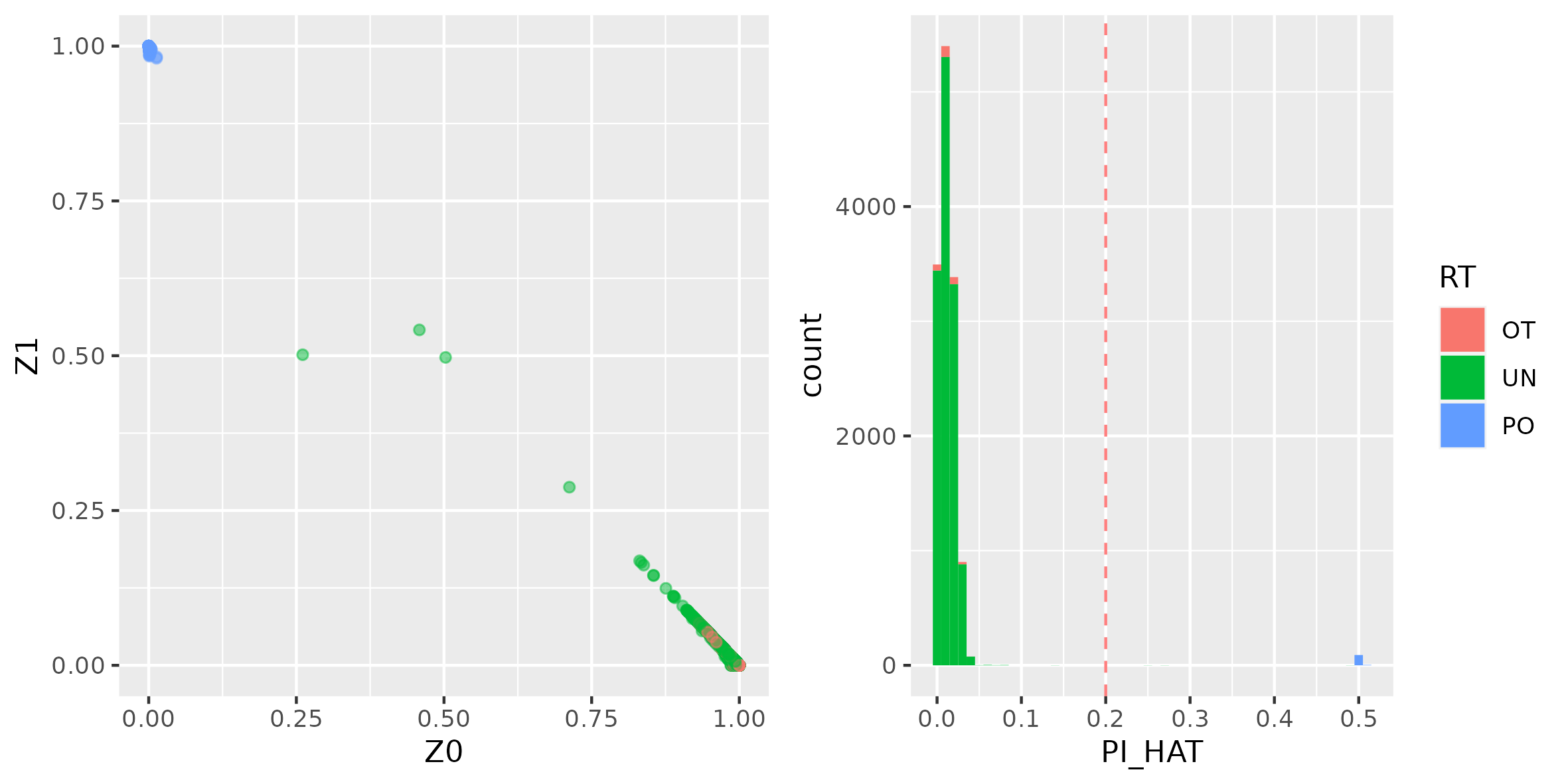
Generated plots show a considerable amount of related individuals in the HapMap data, this is expected since the dataset was constructed as such. As expected, known PO (Parent-Offspring) pair shows highest PI_HAT and Z1 values (ideal parent-offspring has (Z0, Z1, Z2) = (0, 1, 0), i.e. all loci have one allele identical by descent).

Since majority of the relatedness was due to known parent-offspring pairs you can filter your dataset to include only founders (individuals without parents in the dataset) using --filter-founders. This flag will excludes all samples with at least one known parental ID from the current analysis.

plink --bfile hapmap_7 --filter-founders --make-bed --out hapmap_8

Now after keeping only founders let's see if there is any criptic relatedness remaining in our dataset (i.e. pairs of individuals with with a pihat > 0.2).

plink --bfile hapmap_8 --genome -min 0.2 --out hapmap_8.min_pihat_02

We can see that there is still one pair of individuals with pi-hat value higher than 0.2.

We can use the --rel-cutoff flag to remove one of the individuals from the related pairs (in case of multiple related pairs plink will try to maximize the final sample size by prioritizing removal of individuals related to multiple individuals in dataset):

plink --bfile hapmap_8 --rel-cutoff 0.2 --make-bed --out hapmap_9

Congratulations! You've just succesfully completed the first tutorial! You are now able to conduct a proper QC.